Breaking Down Robustness in Robotic Systems
Robustness only becomes visible once the world stops behaving as expected.
In deployment, inputs are imperfect, execution is delayed, hardware behaves inconsistently, and environments differ in ways no benchmark fully captures. A robust model is one that continues to behave sensibly under these conditions—not because the system is clean, but because the model can tolerate messiness.
This post breaks down what we mean by robustness in a robotic policy where it matters, how we think about it, and what categories of failure we use to reason about it before examining specific failure modes in later posts.
Robustness as a property of the model
Robustness is not about constructing a flawless pipeline. Real systems will never be flawless.
Cameras saturate. Sensors drift. Networks lag. Actuators slip. These are not edge cases—they are the normal operating conditions of deployed systems. The question is not whether these failures occur, but whether the model can function despite them.
A robust model maintains useful behavior when parts of the pipeline misbehave. It does not require ideal inputs or perfect execution to succeed. It continues to act appropriately even when observations are distorted, delayed, or incomplete.
The pipeline matters because it is where these failures enter.
The information pipeline
An embodied agent operates as a closed loop between the world and its actions:
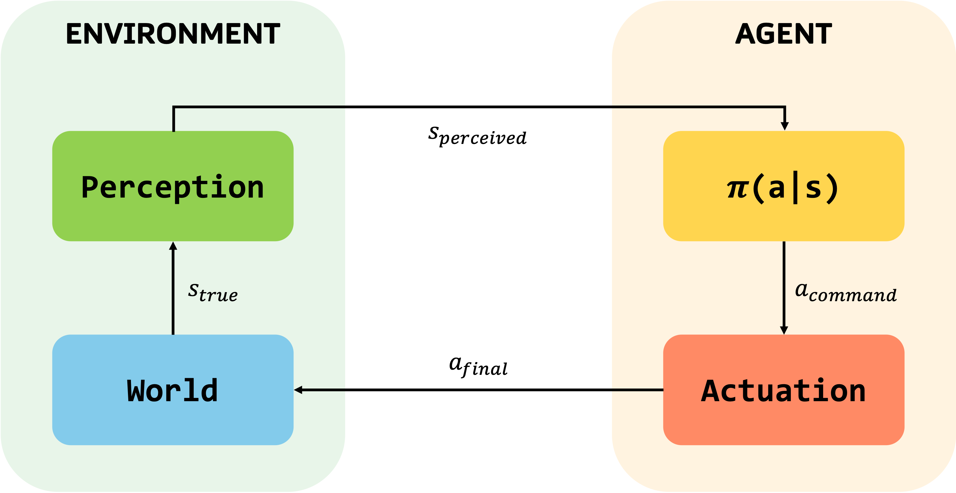
Each stage represents a point where errors can be introduced before the action is ever executed in the environment. Robustness is about whether the model remains reliable as these issues accumulate.
Where perturbations enter the system
Rather than treating robustness as a single axis, we reason about it by looking at where perturbations enter and how they affect the policy.
Note: We intentionally omit reward signals from this diagram. While rewards are central to training, our focus here is on the deployment-time information pipeline—the path from observation to action—where robustness failures manifest in practice.
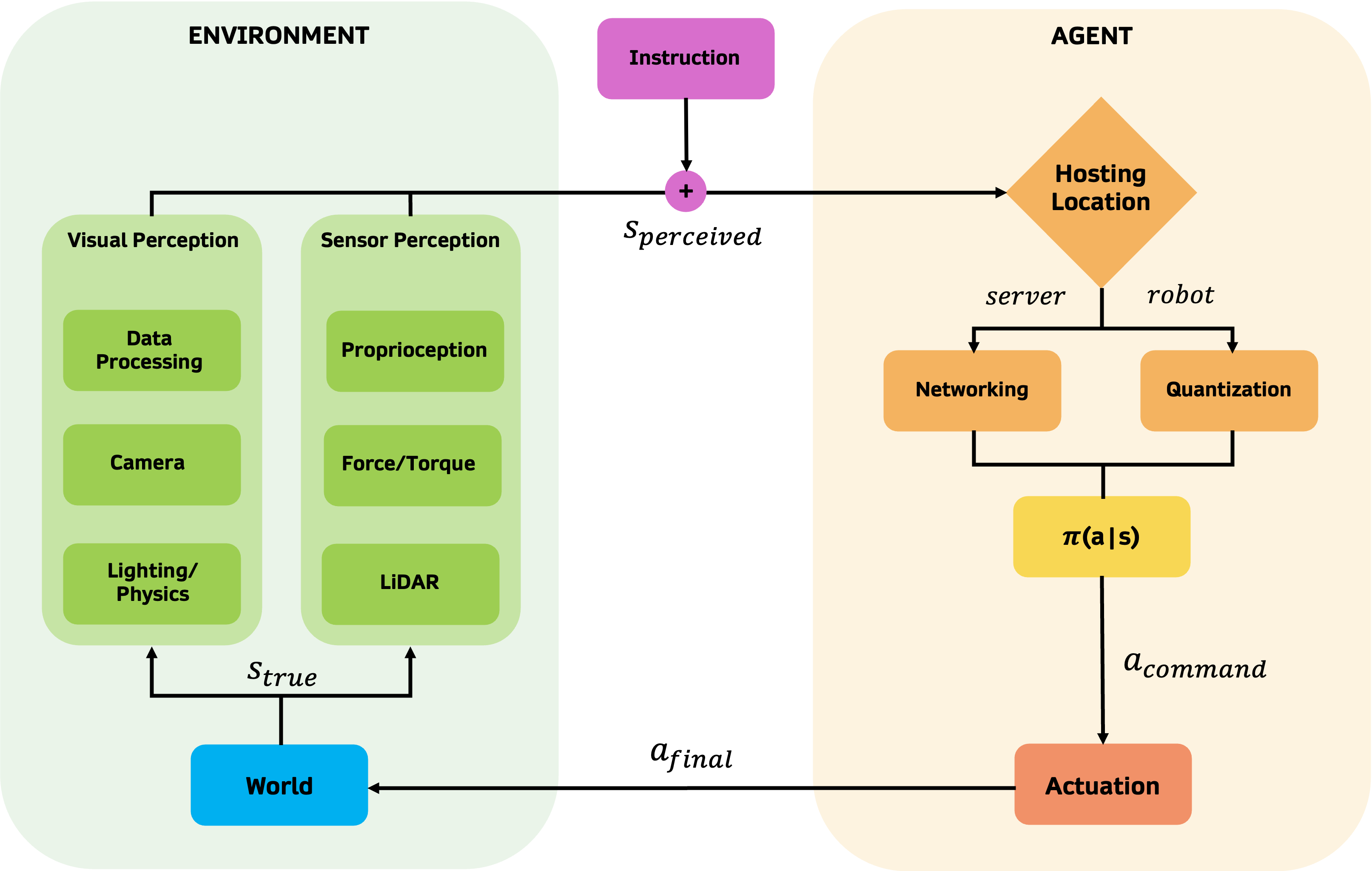
This gap between what a model experiences during training and what it encounters in deployment is closely related to the sim-to-real transfer problem in robotics. In simulation, observations are clean, actions execute perfectly, and conditions are tightly controlled. The real world offers none of these guarantees. The robustness categories we outline below map directly onto the kinds of distributional shifts that make sim-to-real transfer difficult—degraded perception, ambiguous instructions, constrained compute, and imprecise actuation are all faces of the same underlying challenge.
These groupings are not meant to be exhaustive, but rather an overview of the primary failure modes we see repeatedly in practice.
Perception-related perturbations
Perception is where the physical world is converted into model inputs. Failures here tend to arise from ordinary deployment conditions such as: lighting that differs from training data, motion that introduces blur, compression added for bandwidth constraints, or sensors whose characteristics change over time.
The model never observes the world directly. It observes a representation shaped by optics, preprocessing, and hardware. Robustness at this stage is about whether the model can still infer the relevant state when that representation is degraded.
Below we show an example of a model breaking down when motion blur is introduced.
Instruction and semantic perturbations
Modern generalized models typically accept high-level instructions. Here, the challenge is not physical noise but semantic variation such as: users phrasing the same intent differently, context being omitted, underspecified goals or even instructions that conflict with the current state of the environment.
A robust model should behave consistently across such variations. It should not depend on narrow phrasing or a single canonical instruction format to operate correctly. At the same time, this raises an important question: to what extent does the model truly condition on the instruction it is given? If altering phrasing, structure, or wording does not meaningfully influence behavior, what does that imply about how instructions are being interpreted?
Below you’ll see an example of a model that is not robust when a large number of words are swapped for their synonyms.
Compute and hosting perturbations
Where and how the policy runs also matters. A model deployed on a server is subject to latency and network variability. A model deployed on a robot must operate under memory limits, reduced numerical precision, and fixed control rates.
In some cases, deployment involves modifying the model itself—for example through quantization—to meet hardware constraints. Below we show how this can degrade model performance.
In practice, these constraints force real tradeoffs between where a policy runs and how it is represented. Simulation often assumes instantaneous inference with full-precision models, but real systems must choose between network latency and model compression. Unfortunately, neither comes for free.
Actuation and embodiment perturbations
Finally, actions must be executed in the physical world. Motors are imperfect. Contacts are uncertain. Calibration drifts. Surfaces vary. Even when the policy produces the correct command, the outcome may differ from what was intended. Even something as simple as a delay in acting can cause model performance to degrade:
Robust models do not assume perfect execution. They recover from small execution errors, avoid unstable correction loops, and prevent minor deviations from cascading into failure.
Why we study these separately
In deployment, these perturbations rarely appear in isolation, so why are we going to evaluate them independently over the next few blogs?
Studying each category independently allows us to isolate sensitivity along a single dimension. It establishes baselines for how the model responds when one part of the system degrades while others remain stable. Without this, multi-factor failures become difficult to interpret. When everything breaks at once, it becomes unclear which sensitivities matter and which are incidental.
This isolation is what makes later analysis of interacting failures meaningful.